
Ever wondered what your utility bill was going to be before you got it? Or wanted to see your utility usage live? Well you’re in luck, because most utility meters nowadays typically transmit this data over radio frequencies (RF) or cellular. In the case of cellular, your utility company probably already has a fairly up to date dashboard of your usage. But in the case of RF, your utility company still has to have someone get close-ish to the meter to read it. They usually do this by just driving around the neighborhood once a month. The focus of this article is going to be on reading RF based utility meters.
My gas meter transmits over RF, and the meter reader car only comes by once a month to get an accurate reading for the bill, which just wasn’t good enough for me. I want to see in relatively live time what my gas usage is, primarily in the winter. There’s really not that much to reading these meters if you have some technical chops. If you don’t have some technical chops, this article isn’t going to be a step by step guide, but it’ll provide you with an outline and you can google the rest.
Radio
For the actual radio part of this project, I’m using a NooElec USB stick with a small antenna fixed to it (https://www.nooelec.com/store/). I’ve generally found this to be a really cool product, with a lot of open source tooling out there to play around with it, and at a reasonable price.
If you do end up going this route, one thing I tripped up on with the NooElec USB stick was installing the drivers. Make sure you read the instructions for installing the drivers and don’t spend 3 hours trying to figure out why it won’t work before reading the instructions like I did…
Software
There’s a few parts to this. Before you even read further, install Golang (a.k.a Go). Once you have Go installed, you’ll need to install rtl-sdr and rtl-amr. Instructions for both of those can be found at https://github.com/bemasher/rtlamr. We need rtl-sdr for a specific command it provides, rtl-tcp, which is sort of like a server for controlling rtl-sdr programmatically. Then rtl-amr is what actually communicates with rtl-tcp to tell rtl-sdr what frequencies to listen on and then decode the data packets read from the gas meter.
Since we want to store this data so we can later view it in Grafana, we also need another piece called rtlamr-collect which can be found at https://github.com/bemasher/rtlamr-collect. This takes the data rtl-amr spits out and sends it to our InfluxDB database, which we’ll get to in a bit.
The command for starting rtl-tcp is pretty straightforward, just open a command prompt or terminal and enter:
rtl_tcp

// If it gets mad and says it can't find it, specify the absolute path to it like so
C:\Users\Techetio\go\bin\rtl_tcp
Once rtl-tcp is up and running, we can open a new command prompt window to start rtl-amr, and optionally rtlamr-collect like so:
C:\Users\Techetio\go\bin\rtlamr -msgtype=scm+ -format=json -filterid=12345678 | C:\Users\Techetio\go\bin\rtlamr-collect The main things to note here are that the msgtype argument will vary depending on your meter, and the filterid argument will be the 8 digit ID listed on your meter. To use rtl-collect, you just pipe the output of rtl-amr (it has to be json) to the rtlamr-collect process. One big caveat to this is that rtlamr-collect doesn’t take arugments, but rather reads environment variables, and we haven’t set those yet. So you need to go back to the github page for rtlamr-collect to grab the names of the environment variables you’ll need to create. The values of the environment variables will be from the InfluxDB instance we’ll set up in the next section.
InfluxDB
We’ll need InfluxDB running so we have a place to send our metrics to for storage, and a place for Grafana to query our metrics from. I’m a fan of Docker and containerization in general, so I’m running InfluxDB in Docker using the below command:
docker run -d --name influxdb -p 8086:8086 influxdbOnce we have it running on our machine, we can then go to http://localhost:8086/ to do the initial set up. The main things to note are the organization name you set and the bucket name. You’ll also need to make a read/write token for rtlamr-collect and Grafana to use. This can be created under the Data tab, and then the Token tab. Now that you have this information, set the environment variables for rtlamr-collect, and if you already have it running, you’ll need to restart it for the changes to take effect.
Grafana
Now we can set up Grafana to actually visualize the data. Once again I’m running Grafana in Docker with a command similar to below:
docker run -d -p 3000:3000 --name grafana --env GF_AUTH_BASIC_ENABLED=false --env GF_AUTH_DISABLE_LOGIN_FORM=true --env GF_AUTH_DISABLE_SIGNOUT_MENU=true --env GF_AUTH_ANONYMOUS_ENABLED=true --env GF_AUTH_ANONYMOUS_ORG_ROLE=Admin grafana/grafanaThe environment variables are more or less to disable authentication on Grafana so I don’t have to login, because after all this is just running on my local machine.
With Grafana up and running, we can head to http://localhost:3000 to start configuring it. First we need to add the InfluxDB datasource, so we’ll head over to the datasources tab and add a new Influx data source. Because I’m using Docker for Grafana, we have to tell it to use the underlying host’s networking, so the address for InfluxDB will be http://host.docker.internal:8086/. We can then enter the same information as we entered into our environment variables for rtlamr-collect.
With the datasource up and running, lets create a new dashboard, add a panel, and edit the panel. We first need to set the datasource to our new Influx datasource, and then we can add a Flux query that looks something like this to start displaying how many therms we’re using:
from(bucket: "Utilities")
  |> range(start: v.timeRangeStart, stop: v.timeRangeStop)
  |> filter(fn: (r) => r["_measurement"] == "utilities")
  |> filter(fn: (r) => r["_field"] == "consumption")
  |> filter(fn: (r) => r["endpoint_id"] == "12345678")
  |> aggregateWindow(every: v.windowPeriod, fn: mean, createEmpty: false)
  |> derivative(unit: 1m)
  |> map(fn: (r) => ({
      r with
      _value: r._value / 100.0
  }))
  |> yield(name: "mean")
Make sure you update your bucket name, the measurement name you set, and the endpoint ID with the ID of your meter. The rest can stay the same. With that, you should have data points start popping up on your chart.
Another query I like is one that shows my therms usage over the past hour, day, week, month, or whatever time frame you choose. The best panel type for this one is stat or gauge:
from(bucket: "Utilities")
  |> range(start: v.timeRangeStart, stop: v.timeRangeStop)
  |> filter(fn: (r) => r["_measurement"] == "utilities")
  |> filter(fn: (r) => r["_field"] == "consumption")
  |> filter(fn: (r) => r["endpoint_id"] == "12345678")
  |> map(fn: (r) => ({
      r with
      _value: float(v: r._value) / 100.0
  }))
  |> difference(columns: ["_value"])
  |> cumulativeSum()
And to add onto the above query, if you know the price per therm of your gas bill, you can modify this query a little bit to have a panel show the price instead of the therms.
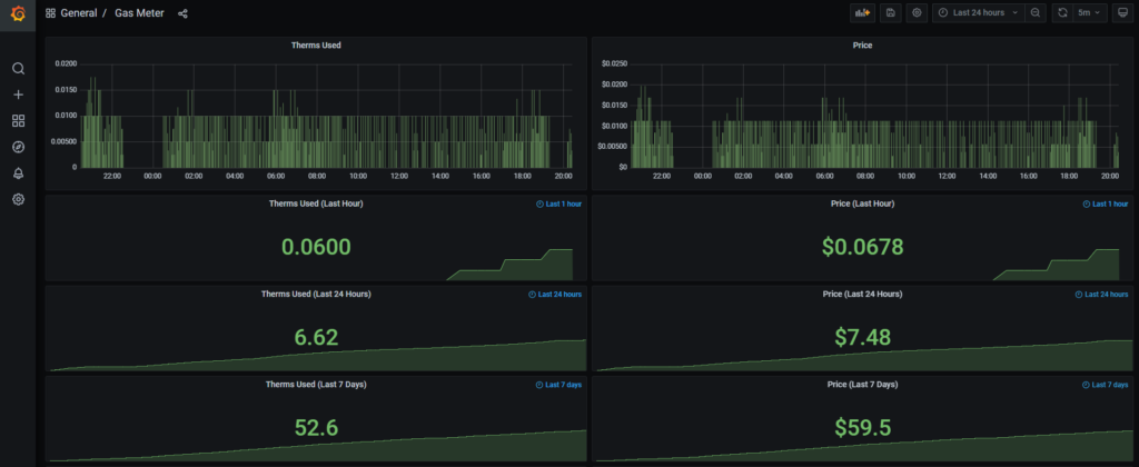
My latest iteration of the dashboard currently looks something like this. There’s a lot of improvements I’ll be making to this in the future to make it look fancier, but for now it’s functional. You can even see when my thermostat schedule changes the temperature. There’s no usage where the furnace was shut off to lower the temperature at night and a noticeable increase in usage many hours later in the morning when the temperature was increased.
The Grafana dashboard json can be found here.
You should share the dashboard json as well, I would love to see how you setup some of the graphs
I went ahead and threw a link to the json at the end of the article here. You’ll likely still have to go in and change certain things. I think there’s several panels where I still have the therms price from last year hard coded in.